DuckDB - Bringing Big Data To Your Laptop
Table of Contents
TL;DR: DuckDB is online analytical processing (OLAP) database management system with a python library providing the ability to quickly perform initial Extract Transform Load (ETL) steps on larger than memory datasets without having to resort to heavier solutions like Hadoop/Spark. It’s a useful tool to extend analysis typically performed in pandas to larger collections of data, especially in parquet format.
Exploring DuckDB - Tons of Taxis
This post documents an exploratory analysis of the DuckDB python library to process big data (roughly defined as data which is too large to fit into memory). The candidate dataset used is the great info on taxi trips provided by the New York City Taxi and Limousine Commission. The data is in parquet format, which is an open source column based format “designed for efficent data storage and retrieval”.
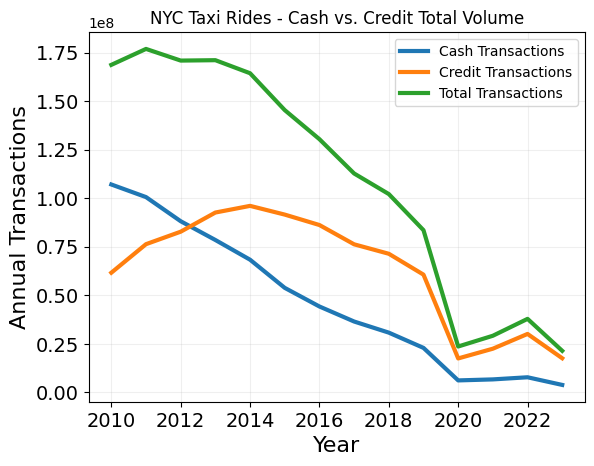
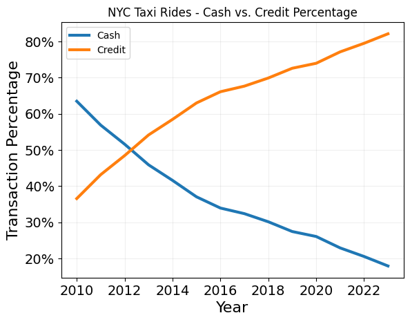
In this exploration, I look at the evolution of fare and payment type for NYC yellow taxis from 2009 to present day using DuckDB. While the results are not too surprising (fares are more expensive, more people use credit cards than cash now, and total number of yellow taxis rides is on the decline), I came away very impressed with the performance of DuckDB queries and the usefulness of its python package.
Import DuckDB and other python libraries
import duckdb
import matplotlib.pyplot as plt
from matplotlib.ticker import PercentFormatter
import matplotlib.pylab as pl
import pandas as pd
import time
import urllib
import os.path
import numpy as np
Getting the Data
Data from https://www.nyc.gov/site/tlc/about/tlc-trip-record-data.page is provided on a monthly basis all the way back to 2009. Investigating the url’s from the website, we can see that they follow the format https://d37ci6vzurychx.cloudfront.net/trip-data/yellow_tripdata_<YYYY>-<MM>.parquet, where <YYYY> is the year (e.g. 2021) and <MM> is the month (e.g. 02 for February). So first let’s make a pandas dataframe which stores the appropriate link, month, and year.
Create dataframe relate links to months/years
# Utilize the % operator for sprintf like formatting
BASE_URL = "https://d37ci6vzurychx.cloudfront.net/trip-data/yellow_tripdata_%d-%02d.parquet"
taxi_years = list(range(2009,2024,1))
months_as_nums =  list(range(1,13,1))

taxi_links = []
for year in taxi_years:
    for month in months_as_nums:
        taxi_links.append(
            {
                'year':year,
                'month':month,
                'data_url':BASE_URL % (year,month)
            }
        )

taxi_df = pd.DataFrame.from_records(taxi_links)

#Remove months that aren't available online/haven't happened yet
taxi_df = taxi_df[~((taxi_df['year']==2023) & (taxi_df['month']>7))]
taxi_df.head()
| year | month | data_url | |
|---|---|---|---|
| 0 | 2009 | 1 | https://d37ci6vzurychx.cloudfront.net/trip-data/yellow_tripdata_2009-01.parquet |
| 1 | 2009 | 2 | https://d37ci6vzurychx.cloudfront.net/trip-data/yellow_tripdata_2009-02.parquet |
| 2 | 2009 | 3 | https://d37ci6vzurychx.cloudfront.net/trip-data/yellow_tripdata_2009-03.parquet |
| 3 | 2009 | 4 | https://d37ci6vzurychx.cloudfront.net/trip-data/yellow_tripdata_2009-04.parquet |
| 4 | 2009 | 5 | https://d37ci6vzurychx.cloudfront.net/trip-data/yellow_tripdata_2009-05.parquet |
Downloading the Data
Here's the code to download the data to the local folder. Local paths are added to taxi_df dataframe in the filename column.
Next step is to download the data using the urllib package. Th below code downloads the data to the current folder with the same naming convention as provided by the NYC Taxi & Limousine Commision.
for url in taxi_df.data_url:
    #check to see if file is downloaded in-case rerunning script
    if not(os.path.isfile(url.split('/')[-1])):
        urllib.request.urlretrieve(url, url.split('/')[-1])
The local files can also be added to pandas dataframe used to track the urls.
taxi_df['filename'] = [url.split('/')[-1] for url in taxi_df.data_url]
Once the data is downloaded, we can check the total size of the dataset by accessing the parquet metadata, more info available here.
total_size_GB = duckdb.execute(f"""
SELECT SUM(total_compressed_size)/(1024*1024*1024) FROM parquet_metadata({list(taxi_df.filename)})
""").fetchall()[0][0]

total_size_uncompressed_GB = duckdb.execute(f"""
SELECT SUM(total_uncompressed_size)/(1024*1024*1024) FROM parquet_metadata({list(taxi_df.filename)})
""").fetchall()[0][0]

print(f"Total size of all files (compressed size): \t {total_size_GB:.2f} GB")
print(f"Total uncompressed size (pandas in memory): \t {total_size_uncompressed_GB:.2f} GB")
Total size of all files (compressed size): 	 27.99 GB
Total uncompressed size (pandas in memory): 	 59.40 GB
With a total size of all files about 28 GB, this dataset is too large to store in memory (at least on my personal computer). Especially since the uncompressed size is over twice that size at 59.4 GB. It also highlights that parquet is a compressed data format, which can save disk space for columns with many repeating or empty values.
Investigate Columns - What’s The Data?
With the data downloaded, let’s take look at the schema and see if it is consistent across all of the parquet files. If the schema does differ, DuckDB provides the ability to handling unions, with either union_by_name or union_by_position (see more here).
col_vals = duckdb.execute(f"""
SELECT file_name, path_in_schema FROM parquet_metadata({list(taxi_df.filename)})
""").df()
We can see which columns are available in each dataset. Let’s group by case insensitive column names, since SQL column variables are case insensitive.
grouped_col_names = col_vals.groupby(col_vals['path_in_schema'].str.lower())\
                            .agg(['unique'])\
                            .reset_index()
grouped_col_names.head()
| path_in_schema | file_name | path_in_schema | |
|---|---|---|---|
| unique | unique | ||
| 0 | __index_level_0__ | [yellow_tripdata_2010-02.parquet, yellow_tripd... | [__index_level_0__] |
| 1 | airport_fee | [yellow_tripdata_2011-01.parquet, yellow_tripd... | [airport_fee, Airport_fee] |
| 2 | congestion_surcharge | [yellow_tripdata_2011-01.parquet, yellow_tripd... | [congestion_surcharge] |
| 3 | dolocationid | [yellow_tripdata_2011-01.parquet, yellow_tripd... | [DOLocationID] |
| 4 | dropoff_datetime | [yellow_tripdata_2010-01.parquet, yellow_tripd... | [dropoff_datetime] |
And we can find the coverage of variable names across datasets by checking which files each column appears in.
all_files = set(taxi_df.filename.values)

coverage =  [
    len(
        all_files.intersection(set(grouped_col_names['file_name']['unique'].iloc[i]))
    )/len(all_files)
    for i in range(grouped_col_names.shape[0])
]
grouped_col_names['coverage'] = coverage
We can see columns that appear in the largest fraction of parquet files.
grouped_col_names.sort_values(by='coverage',ascending=False).head(10)
| path_in_schema | file_name | path_in_schema | coverage | |
|---|---|---|---|---|
| unique | unique | |||
| 35 | trip_distance | [yellow_tripdata_2009-01.parquet, yellow_tripd... | [Trip_Distance, trip_distance] | 1.000000 |
| 15 | payment_type | [yellow_tripdata_2009-01.parquet, yellow_tripd... | [Payment_Type, payment_type] | 1.000000 |
| 14 | passenger_count | [yellow_tripdata_2009-01.parquet, yellow_tripd... | [Passenger_Count, passenger_count] | 1.000000 |
| 13 | mta_tax | [yellow_tripdata_2009-01.parquet, yellow_tripd... | [mta_tax] | 1.000000 |
| 10 | fare_amount | [yellow_tripdata_2010-01.parquet, yellow_tripd... | [fare_amount] | 0.931429 |
| 27 | tip_amount | [yellow_tripdata_2010-01.parquet, yellow_tripd... | [tip_amount] | 0.931429 |
| 25 | store_and_fwd_flag | [yellow_tripdata_2010-01.parquet, yellow_tripd... | [store_and_fwd_flag] | 0.931429 |
| 31 | total_amount | [yellow_tripdata_2010-01.parquet, yellow_tripd... | [total_amount] | 0.931429 |
| 29 | tolls_amount | [yellow_tripdata_2010-01.parquet, yellow_tripd... | [tolls_amount] | 0.931429 |
| 21 | ratecodeid | [yellow_tripdata_2011-01.parquet, yellow_tripd... | [RatecodeID] | 0.862857 |
And those appearing the smallest fraction of parquet files.
grouped_col_names.sort_values(by='coverage',ascending=False).tail(10)
| path_in_schema | file_name | path_in_schema | coverage | |
|---|---|---|---|---|
| unique | unique | |||
| 7 | end_lat | [yellow_tripdata_2009-01.parquet, yellow_tripd... | [End_Lat] | 0.068571 |
| 30 | tolls_amt | [yellow_tripdata_2009-01.parquet, yellow_tripd... | [Tolls_Amt] | 0.068571 |
| 8 | end_lon | [yellow_tripdata_2009-01.parquet, yellow_tripd... | [End_Lon] | 0.068571 |
| 28 | tip_amt | [yellow_tripdata_2009-01.parquet, yellow_tripd... | [Tip_Amt] | 0.068571 |
| 11 | fare_amt | [yellow_tripdata_2009-01.parquet, yellow_tripd... | [Fare_Amt] | 0.068571 |
| 16 | pickup_datetime | [yellow_tripdata_2010-01.parquet, yellow_tripd... | [pickup_datetime] | 0.068571 |
| 17 | pickup_latitude | [yellow_tripdata_2010-01.parquet, yellow_tripd... | [pickup_latitude] | 0.068571 |
| 24 | store_and_forward | [yellow_tripdata_2009-01.parquet, yellow_tripd... | [store_and_forward] | 0.068571 |
| 23 | start_lon | [yellow_tripdata_2009-01.parquet, yellow_tripd... | [Start_Lon] | 0.068571 |
| 0 | __index_level_0__ | [yellow_tripdata_2010-02.parquet, yellow_tripd... | [__index_level_0__] | 0.011429 |
For reference the most recent documentation of the schema is provided by the NYC Taxi and Limousine Comission here, but it is obvious from the above investigation that this schema has changed over time.
DuckDB Queries
Up until now I’ve been dealing with the metadata of parquet files, which can be read into memory without reading in the entire parquet file. So the following demonstrations are the first which would be difficult to perform with this large of a dataset on a single machine without a streaming approach.
Number of entries
First we can do a quick count of how many rows we have in all of our parquet files
total_rows = duckdb.execute(f"""
SELECT COUNT(*) FROM read_parquet({list(taxi_df.filename)})
""").fetchall()[0][0]

print(f"Total number of rows {total_rows:.2e}")
Total number of rows 1.72e+09
So we have over one billion records of taxi trips over the past 14 years. That’s a lot of taxi rides!
Aggregation Methods
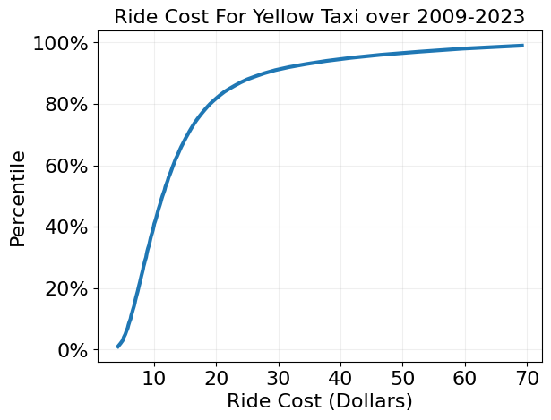
Next let’s get percentiles on the total_amount field. DuckDB has a collection of aggregation functions which perform calculations in parallel as the data is scanned, which does not require loading the full dataset into memory. We’ll start off with the approx_quantile method, which calculates quantiles using the new T-Digest method.
Since total_amount is not present in all parquet files, we need to pass the union_by_name=true to the read_parquet method.
# disable so it doesn't show up in markdown after nbconvert
duckdb.execute("PRAGMA disable_progress_bar;");
percentiles = np.linspace(0.01,0.99,num=99)
total_amount_pctiles = duckdb.execute(f"""
SELECT approx_quantile(total_amount,[{",".join([str(x) for x in percentiles])}])
FROM read_parquet({list(taxi_df.filename)},union_by_name=true)
WHERE total_amount > 0
""").fetchall()[0][0]
Plot distribution of ride costs over entire dataset
plt.plot(total_amount_pctiles,percentiles,linewidth=3)
plt.xlabel('Ride Cost (Dollars)',size=16)
plt.ylabel('Percentile',size=16)
plt.grid(alpha=0.2)
plt.xticks(fontsize=16)
plt.yticks(fontsize=16)
plt.gca().yaxis.set_major_formatter(PercentFormatter(1))
plt.title('Ride Cost For Yellow Taxi over 2009-2023', size=16)
plt.show()

View evolution of ride cost on a per year basis
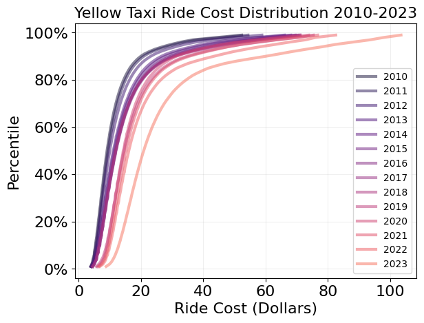
With that out of the way, we can use the year information in the filename to plot the evolution of the cost of ride cost over the years
pcts_over_years = dict()
for year in range(2010,2024,1):
    year_fnames = taxi_df[taxi_df['year']==year]['filename']
    year_pcts = duckdb.execute(f"""
    SELECT approx_quantile(total_amount,[{",".join([str(x) for x in percentiles])}])
    FROM read_parquet({list(year_fnames)},union_by_name=true)
    WHERE total_amount > 0""").fetchall()[0][0]
    year_dict = { str(year):year_pcts }
    pcts_over_years = dict(pcts_over_years, **year_dict)
Plot total fare distribution per year
colors = pl.cm.magma(np.linspace(.1,.7,len(pcts_over_years.keys())))

for idx, year in enumerate(pcts_over_years):
    plt.plot(pcts_over_years[year],percentiles,label=year,alpha=0.5,color=colors[idx],linewidth=3)

plt.title('Yellow Taxi Ride Cost Distribution 2010-2023',size=16)
plt.xlabel('Ride Cost (Dollars)',size=16)
plt.ylabel('Percentile',size=16)
plt.grid(alpha=0.2)
plt.xticks(fontsize=16)
plt.yticks(fontsize=16)
plt.gca().yaxis.set_major_formatter(PercentFormatter(1))
plt.legend()
plt.show()

The above plot shows that the nominal cost of yellow taxi rides in NYC has steadily rising, but has increased significantly in the year 2023. This fits with the trend of higher inflation over the past couple years. If we wanted to investigate the breakdown of the total fare over time (taxes, tips, fees, etc.), those columns are in the dataset as well.
Payment Types
Now let’s look at the counts of different payment types
payment_type_counts = duckdb.execute(f"""
SELECT payment_type, COUNT(*) as occurrence_count
FROM read_parquet({list(taxi_df.filename)},union_by_name=true)
GROUP BY payment_type; """).df()
payment_type_counts.sort_values(by=['occurrence_count'],ascending=False)
| Payment_Type | occurrence_count | |
|---|---|---|
| 5 | 1 | 821291745 |
| 18 | 2 | 548052362 |
| 20 | CASH | 69117503 |
| 17 | Cash | 56282593 |
| 6 | CSH | 50210641 |
| 3 | Credit | 42561382 |
| 12 | CRD | 30829647 |
| 4 | CAS | 30792977 |
| 16 | Cre | 27416855 |
| 2 | Cas | 26058725 |
| 19 | 0 | 4773430 |
| 13 | 3 | 4440736 |
| 0 | CRE | 3370093 |
| 10 | CREDIT | 2330599 |
| 1 | 4 | 1949962 |
| 14 | 5 | 753370 |
| 9 | No Charge | 509194 |
| 22 | No | 200505 |
| 11 | Dispute | 94784 |
| 8 | Dis | 43614 |
| 21 | NA | 40013 |
| 15 | NOC | 31817 |
| 7 | DIS | 6275 |
Like any real dataset, we have some messy data which is the result of human error and changing schemas. Looking at the official documentation, there are currently only six types of payment types with a numerical code for each:
- 1 = Credit
- 2 = Cash
- 3 = No Charge
- 4 = Dispute
- 5 = Unknown
- 6 = Voided Trip
I’m interested in the trends of cash versus credit over time. Let’s hand clean this mess by matching the data to its intended value.
total_cash = duckdb.execute(f"""
SELECT COUNT(*) FROM read_parquet({list(taxi_df.filename)},union_by_name=true)
WHERE payment_type IN (2, 'CASH','Cash','CSH', 'CAS', 'Cas')
""").fetchall()[0][0]

total_credit = duckdb.execute(f"""
SELECT COUNT(*) FROM read_parquet({list(taxi_df.filename)},union_by_name=true)
WHERE payment_type IN (1, 'Credit', 'CRD', 'Cre','CRE', 'CREDIT')
""").fetchall()[0][0]
print(f"""
Total Cash Transactions: \t\t{total_cash:.2e}
Total Credit Transactions: \t\t{total_credit:.2e}
Fraction of Total Transactions: \t{(total_cash+total_credit)/total_rows:.6f}
""")
Total Cash Transactions: 		7.81e+08
Total Credit Transactions: 		9.28e+08
Fraction of Total Transactions: 	0.992538
So there are slighlty more credit tranasctions over the entire dataset than cash transactions. And predictably “Cash or Credit?” corresponding to 99.25% of all transactions. But how the proportion of cash versus credit evolve over time?
years = list(range(2010,2024,1))
cash_years = []
credit_years = []

for year in years:
    year_fnames = taxi_df[taxi_df['year']==year]['filename']

    cash_years.append(
        duckdb.execute(f"""
        SELECT COUNT(*) FROM read_parquet({list(year_fnames)},union_by_name=true)
        WHERE payment_type IN (2, 'CASH','Cash','CSH', 'CAS', 'Cas')
        """).fetchall()[0][0])

    credit_years.append(
        duckdb.execute(f"""
        SELECT COUNT(*) FROM read_parquet({list(year_fnames)},union_by_name=true)
        WHERE payment_type IN (1, 'Credit', 'CRD', 'Cre','CRE', 'CREDIT')
        """).fetchall()[0][0])
Plot "Cash or Credit" annually over dataset"
# Total Transaction Volume
plt.plot(years,cash_years,label='Cash Transactions',linewidth=3)
plt.plot(years,credit_years,label='Credit Transactions',linewidth=3)
plt.plot(years,np.add(cash_years,credit_years),label='Total Transactions',linewidth=3)

plt.xlabel('Year', size=16)
plt.ylabel('Annual Transactions', size=16)
plt.title('NYC Taxi Rides - Cash vs. Credit Total Volume')
plt.legend()
plt.grid(alpha=0.2)
plt.xticks(size=14)
plt.yticks(size=14)
plt.show()

Plot "Cash or Credit" as percentage of all transactions
# Transaction Percentage
plt.plot(years,np.divide(cash_years,np.add(cash_years,credit_years)),label='Cash',linewidth=3)
plt.plot(years,np.divide(credit_years,np.add(cash_years,credit_years)),label='Credit',linewidth=3)

plt.xlabel('Year', size=16)
plt.ylabel('Transaction Percentage', size=16)
plt.title('NYC Taxi Rides - Cash vs. Credit Percentage')
plt.legend()
plt.gca().yaxis.set_major_formatter(PercentFormatter(1))
plt.grid(alpha=0.2)
plt.xticks(size=14)
plt.yticks(size=14)
plt.show()

I’m Different - User Defined Functions
If the SQL queries and DuckDB aggregate functions are not enough for a given use case, DuckDB provides the ability to use User Defined Functions (UDF). With UDF’s, we can define pure python functions that are calculated as the data is continously read. So if the initial aggregation is still too large for memory, we can apply our own defined functions as the data is read in. It is especially cool that we can use third party libraries within the defined function! I’m assuming this works since DuckDB is bound to the particular python process being run.
For this example, let’s do some random math where we take the absolute difference between two values and then calculate the square root with numpy. If we provide type annotation, DuckDB is smart enough to handle the rest. We just need to select columns where both values are not null so the query doesn’t error out.
def random_func(x: float, y: float) -> float:
    return np.sqrt(abs(x-y))

duckdb.create_function('random_func',random_func);
Now let’s use the function in a query by applying the function to the fare_amount and tip_amount method.
random_ans = duckdb.execute(f"""
        SELECT AVG(random_func(fare_amount,tip_amount)) FROM read_parquet({list(taxi_df.filename)},union_by_name=true)
        WHERE tip_amount IS NOT NULL
        AND fare_amount IS NOT NULL
        """).fetchall()[0][0]
print(f"Average value of our random function {random_ans:.2f}")
Average value of our random function 3.07
Introducing this python function did cause the query to be much slower than previous operations. Unlike other queries which quickly brought my CPU usage up to 100%, this one kept my CPU at about 20% for the entire operation. So it is worth trying to avoid python UDFs as the data size becomes large or performance is important.
Final Thoughts
After playing around with DuckDB for a bit, I’m pretty impressed. I think it has an obvious use case for analytical workloads where the data which is larger your computer’s memory, where performance is important, and where its simplicity outweighs potential gains from more heavyweight big data analysis services. Since DuckDB deals with databases in a column based format, I also think it is a natural candidate to process parquet files.
DuckDB Performance
Here are timed benchmarks for all queries performed above. As a reminder, the dataset is 28 GB compressed, 59 GB uncompressed, and has 1.72 billion rows.
These numbers will depend on hardware, so for reference I have a AMD 3600 CPU and the data is stored on a Samsung 970 EVO SSD which has quoted read/write times of 3500 MB/s and 3,300 MB/s respectively. Based on these speeds, I would expect loading in all columns of all parquet files into memory to take at least 28 GB / 3.5 GB/s \(\approx\) 8 seconds if I had that much RAM (which I don’t). Most of the default DuckDB queries which require scanning the all files are on the same time scale of around 10 seconds or less. I’m assuming DuckDB can achieve these times because it can selectively load only the parts of the dataset it needs to execute the query.
Query: Getting total compressed size from parquet metadata
%%timeit

duckdb.execute(f"""
SELECT SUM(total_compressed_size)/(1024*1024*1024) FROM parquet_metadata({list(taxi_df.filename)})
""").fetchall()[0][0]
79.5 ms ± 2.51 ms per loop (mean ± std. dev. of 7 runs, 1 loop each)
Query: Getting total uncompressed size from parquet metadata
%%timeit

duckdb.execute(f"""
SELECT SUM(total_uncompressed_size)/(1024*1024*1024) FROM parquet_metadata({list(taxi_df.filename)})
""").fetchall()[0][0]
82.8 ms ± 2.42 ms per loop (mean ± std. dev. of 7 runs, 10 loops each)
Query: Getting filename and column names from metadata
%%timeit

duckdb.execute(f"""
SELECT file_name, path_in_schema FROM parquet_metadata({list(taxi_df.filename)})
""").df()
78 ms ± 194 µs per loop (mean ± std. dev. of 7 runs, 10 loops each)
Query: Get total number of transactions
%%timeit

duckdb.execute(f"""
SELECT COUNT(*) FROM read_parquet({list(taxi_df.filename)})
""").fetchall()[0][0]
78.1 ms ± 304 µs per loop (mean ± std. dev. of 7 runs, 10 loops each)
Query: Get Approx. Percentiles of Total Amount Column
%%timeit

duckdb.execute(f"""
SELECT approx_quantile(total_amount,[{",".join([str(x) for x in percentiles])}])
FROM read_parquet({list(taxi_df.filename)},union_by_name=true)
WHERE total_amount > 0
""").fetchall()[0][0]
11.5 s ± 19.7 ms per loop (mean ± std. dev. of 7 runs, 1 loop each)
Query: Get Approx Percentiles of Total Amount Column Per Year
%%timeit

pcts_over_years = dict()
for year in range(2010,2024,1):
    year_fnames = taxi_df[taxi_df['year']==year]['filename']
    year_pcts = duckdb.execute(f"""
    SELECT approx_quantile(total_amount,[{",".join([str(x) for x in percentiles])}])
    FROM read_parquet({list(year_fnames)},union_by_name=true)
    WHERE total_amount > 0""").fetchall()[0][0]
    year_dict = { str(year):year_pcts }
    pcts_over_years = dict(pcts_over_years, **year_dict)
12.8 s ± 28.1 ms per loop (mean ± std. dev. of 7 runs, 1 loop each)
Query: Get Number of Transactions Per Payment Type
%%timeit

duckdb.execute(f"""
SELECT payment_type, COUNT(*) as occurrence_count
FROM read_parquet({list(taxi_df.filename)},union_by_name=true)
GROUP BY payment_type; """).df()
5.73 s ± 38.9 ms per loop (mean ± std. dev. of 7 runs, 1 loop each)
Query: Get Number of Cash Transactions Total
%%timeit

total_cash = duckdb.execute(f"""
SELECT COUNT(*) FROM read_parquet({list(taxi_df.filename)},union_by_name=true)
WHERE payment_type IN (2, 'CASH','Cash','CSH', 'CAS', 'Cas')
""").fetchall()[0][0]
6.4 s ± 21.4 ms per loop (mean ± std. dev. of 7 runs, 1 loop each)
Query: Get Number of Credit Transactions Total
%%timeit

duckdb.execute(f"""
SELECT COUNT(*) FROM read_parquet({list(taxi_df.filename)},union_by_name=true)
WHERE payment_type IN (1, 'Credit', 'CRD', 'Cre','CRE', 'CREDIT')
""").fetchall()[0][0]
6.52 s ± 27.8 ms per loop (mean ± std. dev. of 7 runs, 1 loop each)
Query: Get Number of Cash/Credit Transactions Per Year
%%timeit

years = list(range(2010,2024,1))
cash_years = []
credit_years = []

for year in years:
    year_fnames = taxi_df[taxi_df['year']==year]['filename']

    cash_years.append(
        duckdb.execute(f"""
        SELECT COUNT(*) FROM read_parquet({list(year_fnames)},union_by_name=true)
        WHERE payment_type IN (2, 'CASH','Cash','CSH', 'CAS', 'Cas')
        """).fetchall()[0][0])

    credit_years.append(
        duckdb.execute(f"""
        SELECT COUNT(*) FROM read_parquet({list(year_fnames)},union_by_name=true)
        WHERE payment_type IN (1, 'Credit', 'CRD', 'Cre','CRE', 'CREDIT')
        """).fetchall()[0][0])
13.2 s ± 49.9 ms per loop (mean ± std. dev. of 7 runs, 1 loop each)
Query: User Defined Function
#Got impatient since this is a really slow query
from timeit import default_timer as timer

start = timer()
duckdb.execute(f"""
        SELECT AVG(random_func(fare_amount,tip_amount)) FROM read_parquet({list(taxi_df.filename)},union_by_name=true)
        WHERE tip_amount IS NOT NULL
        AND fare_amount IS NOT NULL
        """).fetchall()[0][0]
end = timer()

print(f"User Defined Function Took {end-start:.2e} seconds")
User Defined Function Took 2.09e+03 seconds
Which is about 35 minutes.