Accessing Google's Petabyte Scale Satellite Data

Accessing Satellite Imagery with Google Earth Engine

Satellites provide a wealth of information about the world: monitoring human development, tracking climate change, and providing vital information at scale for disaster response. Over the past decades, the scale of publicly accessible satellite data has increased exponentially. This data is collected by many research consortia, often stored on servers and accessible with APIs unique to the mission. Google’s Earth Engine hosts a large, multi-petabyte catalog of satellite imagery which can be accessed and queried with a common API, for free with a Google account. This service, which requires the technical knowledge and bankroll of a tech giant, is boon for using satellite imagery at scale to learn more about the world we live in. This post documents basic interaction with the Earth Engine API in python, focusing on how to get Sentinel-2 MSI imagery.

# Import Libraries

import ee  # Google Earth Engine
import eemont  # Extension to Google Earth Engine

from PIL import Image
import requests
import rasterio
import numpy as np
import datetime
import geopy
import geopy.distance
import matplotlib.pyplot as plt

Autheticate Google Earth Engine Account

The first step of using Google Earth Engine (after signing up with a google account) is to authenticate your session, which can be done interactively in a jupyter notebook by running the following commands.

ee.Authenticate()
ee.Initialize()

Select Location to Request Imagery

To query satellite imagery of a particular location on earth, we first need to create a Earth Engine Geometry Object. I’ve found the eeMont python package that extends Google Earth Engine to be helpful in exploratory analysis, since it can return a Geometry Point based on a text query. Below is a query for Washington D.C.

point = ee.Geometry.PointFromQuery("Washington DC", user_agent="earth_engine_example")

Which returns a single longitude, latitude pair for Washington D.C., as you would get if the same query was entered into Google Maps.

print(point)

ee.Geometry({
  "functionInvocationValue": {
    "functionName": "GeometryConstructors.Point",
    "arguments": {
      "coordinates": {
        "constantValue": [
          -77.0365427,
          38.8950368
        ]
      }
    }
  }
})

Create Bounding Box Helper Function

For this example, I want to get a subset of Sentinel-2 Image. In requesting an image, it is necessary to request either the scale (i.e. sampling distance of pixel) of the image or the pixel dimensions of the subset. Sentinel-2 MSI Imagery has a 10m resolution, however if I request a full image at that resolution it is too large. And if I request a image with a specified pixel dimension, then the image is downsampled to a worse resolution than the native 10m.

To get an image subset with roughly native resolution, I created a function that makes a bounding box of a specified size centered on an initial latitude and longitude point.

def BBoxFromPoint(bbox_size, lat_point, lon_point):
    """
    bbox_size - either square in km (one value) or two values in NS km, then EW km
    lat_point - lat center of bounding box
    lon_point - lon center of bounding box

    returns ee.Geometry object of bounding box
    """
    if type(bbox_size) == int or type(bbox_size) == float:
        bbox_size = np.array([bbox_size])

    if len(bbox_size) == 1:
        lat_km = bbox_size[0]
        lon_km = bbox_size[0]
    elif len(bbox_size) == 2:
        lat_km, lon_km = bbox_size
    else:
        raise ValueError("bbox_size must be either length 1 or 2")

    origin = geopy.Point(lat_point, lon_point)
    lat_min = (
        geopy.distance.geodesic(kilometers=lat_km / 2).destination(origin, bearing=180)
    )[0]
    lat_max = (
        geopy.distance.geodesic(kilometers=lat_km / 2).destination(origin, bearing=0)
    )[0]
    lon_min = (
        geopy.distance.geodesic(kilometers=lat_km / 2).destination(origin, bearing=270)
    )[1]
    lon_max = (
        geopy.distance.geodesic(kilometers=lat_km / 2).destination(origin, bearing=90)
    )[1]

    return ee.Geometry.BBox(lon_min, lat_min, lon_max, lat_max)

With this information, I created a bounding box of 5.12 km x 5.12 km so that when I ask for a 512 x 512 pixel image it is approximately at the native 10m resolution of Sentinel-2 MSI imagery.

DC_lon, DC_lat = point.coordinates().getInfo()
DC_bbox = BBoxFromPoint(5.12, DC_lat, DC_lon)

DC_bbox.getInfo()

{'geodesic': False,
 'type': 'Polygon',
 'coordinates': [[[-77.06605134109452, 38.87197649154135],
   [-77.00703405890545, 38.87197649154135],
   [-77.00703405890545, 38.91809701712762],
   [-77.06605134109452, 38.91809701712762],
   [-77.06605134109452, 38.87197649154135]]]}

Get Image Collection From Google Earth Engine

With a location selected, the next step of getting imagery from Google Earth Engine is to specify the dataset. Below this is done by running ee.ImageCollection("COPERNICUS/S2_SR_HARMONIZED"). Creating the ImageCollection object does not return the entire dataset (which is a good thing because it is extremely large), but creates a object on the user side which, when prompted by other methods, can make a request of Google’s server. This is detailed in the Client vs. Server section of Google’s documentation.

After creating the ImageCollection object, the data we are interested can be specified with filter functions, in this case filterBounds for images intersecting the Geometry object, filterDate for specifying the date range to look for images, and filter for a generic filter which can query against properties of each image, listed here for Sentinel-2. The last filter selects images with 5% or less cloudy pixels.

DC_collection = (
    ee.ImageCollection("COPERNICUS/S2_SR_HARMONIZED")
    .filterBounds(DC_bbox)
    .filterDate("2020-01-01", "2021-01-01")
    .filter(ee.Filter.lte("CLOUDY_PIXEL_PERCENTAGE", 5))
)

In the above image collection, multiple images will satisfy the geospatial, temporal, and cloud percentage requirements. Therefore, it is necessary to select a single image from the set of qualifying images. A simple way to do that is with the first method, which can be passed into the ee.Image constructor to make an image object.

DC_image = ee.Image(DC_collection.first())

To grab the metadata associated with this image, we need to call the getInfo method on the Image object. This is because the Image object exists on the Client side and has not yet made a request to Google’s servers.

DC_Image_info = DC_image.getInfo()

print("Image Info is a ", type(DC_Image_info))

Image Info is a  <class 'dict'>

print("Fields of Image Info:")
for key in DC_Image_info:
    print(key)

Fields of Image Info:
type
bands
version
id
properties

print("Start time of Image:\t", DC_Image_info["properties"]["system:time_start"])

print(
    "Date:\t\t\t",
    datetime.datetime.fromtimestamp(
        DC_Image_info["properties"]["system:time_start"] / 1000
    ).strftime("%c"),
)

print("Sentinel ID:\t\t", DC_Image_info["properties"]["DATATAKE_IDENTIFIER"])

Start time of Image:	 1579190537887
Date:			 Thu Jan 16 11:02:17 2020
Sentinel ID:		 GS2B_20200116T155609_014952_N02.13

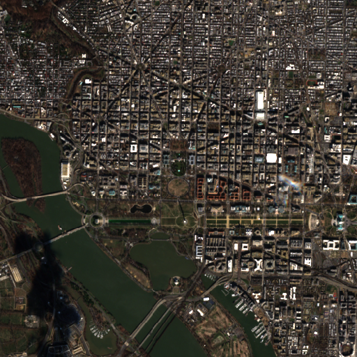
To get the actual image from Google’s servers, you need to call either getThumbURL or getDownloadURL. getThumbURL will generate a url with the image in the requested format. This function requires a dictionary specifying the parameters necessary to generate the image. For instance, Sentinel-2 data has over 10 bands and which band should be mapped to Red, Green, and Blue is ambiguous. Below the bands B4, B3, B2 are mapped red, green, and blue respectively. For multispectral imagery (MSI) these bands correspond to their mapped colors, but for other formats of imagery such as those beyond the visible must be assigned to artificial colors.

In addition to specifying the bands, the pixel dimensions of the image, and the bounding box of the image, the data range of the image needs to be specified. According to the data description on the Google Earth Engine website, the data value of the band is the surface reflectance multiplied by 10,000. I’ve found decent results by setting the data range from $[0,4000]$, or a surface reflectance from 0% to 40%.

The url can be read into a PIL image by using the requests module and passing the raw response into PIL.Image.open().

DC_url = DC_image.getThumbURL(
    {
        "format": "png",
        "bands": ["B4", "B3", "B2"],
        "dimensions": [512, 512],
        "region": DC_bbox,
        "min": 0,
        "max": 4000,
    }
)

DC_thumbURL_response = requests.get(DC_url, stream=True)

DC_PIL = Image.open(DC_thumbURL_response.raw)

DC_PIL

Since the data is in a PIL Image, it can be saved easily with the .save method.

DC_PIL.save("Sentinel-2_DC.png")

Download Image as a GeoTiff

The thumbnails from getThumbURL are meant to be visualized and therefore require either one band (grayscale) or three bands (RGB). However, to get the full data from all or a selection of the bands collected you need to download the GeoTiff with getDownloadURL. The format is very similar to the getThumbURL method as it requires a dictionary specifying parameters of image. Instead of generating a png, the download url is a zip file which unzips into a GeoTiff.

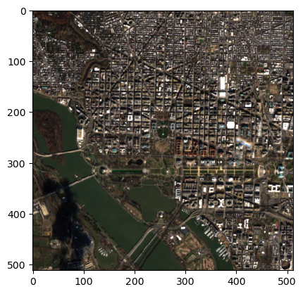
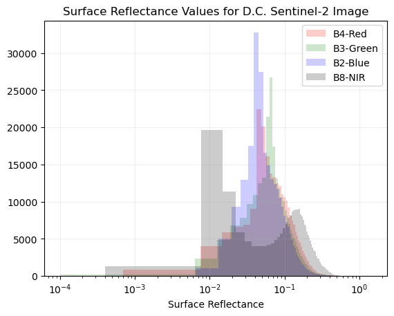
The code below generates the download url, downloads the image, uzips it, loads it with rasterio, and plots the image (same as above) and the histogram of the reflectance values

DC_downloadURL = DC_image.getDownloadURL(
    {
        "bands": ["B2", "B3", "B4", "B8"],
        "dimensions": [512, 512],
        "region": DC_bbox,
        "filePerBand": False,
    }
)

DC_download_response = requests.get(DC_downloadURL)

with open("DC_geotiff.zip", "wb") as fd:
    fd.write(DC_download_response.content)

import zipfile

with zipfile.ZipFile("DC_geotiff.zip", "r") as zip_ref:
    zip_ref.extractall()

import glob

fname = glob.glob("*.tif")

DC_dataset = rasterio.open(fname[0])

print("Image heigt, width:", DC_dataset.height, ",", DC_dataset.width)
print("Number Bands:", DC_dataset.count)
print("Datatype:", DC_dataset.dtypes[0])

Image heigt, width: 512 , 512
Number Bands: 4
Datatype: uint16

DC_raster = DC_dataset.read([3, 2, 1])

Warning 1: TIFFReadDirectory:Sum of Photometric type-related color channels and ExtraSamples doesn't match SamplesPerPixel. Defining non-color channels as ExtraSamples.

plt.imshow(np.moveaxis(DC_raster, 0, -1) / np.percentile(DC_raster, 99))

And with the full range of the bands, which are processed to be in units of surface reflectance multiplied by 10,000, the histogram of the selected bands can be plotted. Notably, the GeoTiff bands have a much larger dynamic range (16-bit) versus the png image returned from getThumbUrL (8-bit).

# Red band
plt.hist(
    (DC_dataset.read(3).flatten()) / 10000, 200, color="red", alpha=0.2, label="B4-Red"
)

# Blue band
plt.hist(
    (DC_dataset.read(2).flatten()) / 10000,
    200,
    color="green",
    alpha=0.2,
    label="B3-Green",
)

# Green band
plt.hist(
    (DC_dataset.read(1).flatten()) / 10000,
    200,
    color="blue",
    alpha=0.2,
    label="B2-Blue",
)

# NIR band
plt.hist(
    (DC_dataset.read(4).flatten()) / 10000,
    200,
    color="black",
    alpha=0.2,
    label="B8-NIR",
)

plt.xscale("log")
plt.xlabel("Surface Reflectance")
plt.grid(alpha=0.2)
plt.title("Surface Reflectance Values for D.C. Sentinel-2 Image")
plt.legend()
plt.show()

Generate timelapse video

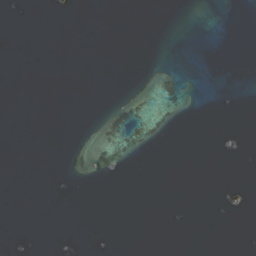
As an example of the power and flexibility of Google Earth Engine, here is a quick script to save frames for a timelapse video of the construction of Fiery Cross Reef, a coral reef in the South China Sea which was terraformed by China into a naval base from 2013 to 2017.

Generate movie of Fiery Cross Reef construciton

fcr_bbox = BBoxFromPoint(0.03 * 256, 9.549167, 112.889167)

fcr_collection = (
    ee.ImageCollection("LANDSAT/LC08/C02/T1_L2")
    .filterBounds(fcr_bbox)
    .filterDate("2013-04-01", "2018-06-01")
    .filter(ee.Filter.lte("CLOUD_COVER", 50))
)

# test the example image

fcr_first_image = ee.Image(fcr_collection.first())

fcr_url = fcr_first_image.getThumbURL(
    {
        "format": "png",
        "bands": ["SR_B4", "SR_B3", "SR_B2"],
        "dimensions": [256, 256],
        "region": fcr_bbox,
        "min": 0,
        "max": 29000,
    }
)

fcr_first_response = requests.get(fcr_url, stream=True)

fcr_PIL = Image.open(fcr_first_response.raw)

fcr_PIL

# Loop through the images and save them

number_of_images = fcr_collection.size().getInfo()
fcr_list = fcr_collection.toList(fcr_collection.size())

for i in range(number_of_images):
    fcr_image = ee.Image(fcr_list.get(i))

    fcr_url = fcr_image.getThumbURL(
        {
            "format": "png",
            "bands": ["SR_B4", "SR_B3", "SR_B2"],
            "dimensions": [256, 256],
            "region": fcr_bbox,
            "min": 0,
            "max": 30000,
        }
    )

    fcr_response = requests.get(fcr_url, stream=True)
    fcr_PIL = Image.open(fcr_response.raw)

    fcr_PIL.save(f"fcr_images/fcr_{i:03}.png")

With the images are combined into mp4 using ffmpeg.